|
Spline Representations I
I google
“spline” and I get http://www.mathworks.com/products/splines/
as the second hit (the first hit brings up a university site that informs me
how I don’t have access to it
A better link is http://www.saltire.com/applets/advanced_geometry/spline/spline.htm which is a very nice interactive applet with a succinct explanation of spline it illustrates.
Here’s another good one: http://www.math.ucla.edu/~baker/java/hoefer/Spline.htm .
Splines were invented out of a need to draw approximating curves with a minimum of computation. Most students first get a hint of this when they study Simpson’s method in calculus. With Simpson’s method a function is sampled and the samples are grouped to fit parabolas to adjacent sets of three and the area under the curve can be approximated as the sum of areas under the adjacent parabolas, which, after considerable simplification, comes to the simple formula The simplest sort of splines typically takes up where this leaves off: by fitting a cubic to adjacent sets of three, with the added condition that the slopes of the tangent lines to the curve and the approximating cubic agree at the splice, so the curve is smooth throughout.
OpenGL’s
If we parameterize a space curve we can impose parametric continuity conditions by equating parametric derivatives of adjacent curve sections at their common boundary.
The zero-order continuity condition, C0, is simply that the curves connect; that the right endpoint of one section meets the left endpoint of the next section: v(t2) = v(t1). The first-order continuity condition requires that the tangent line (directional derivatives) agree. The second-order continuity condition requires that the curves meet and the 1st and 2nd order parametric derivatives agree.
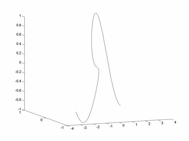
Example The vector valued space curve
t = -pi:pi/50:pi;
and then plot the space curve using these commands (“real” is needed to force the real root):
plot3(t,sin(real(t^(2/3))),sin(real(t^(4/3)))) axis square grid on
the plot can then be rotated by clicking and dragging on it. From this perspective, it looks pretty smooth, though there is evidence of a kink at the origin.
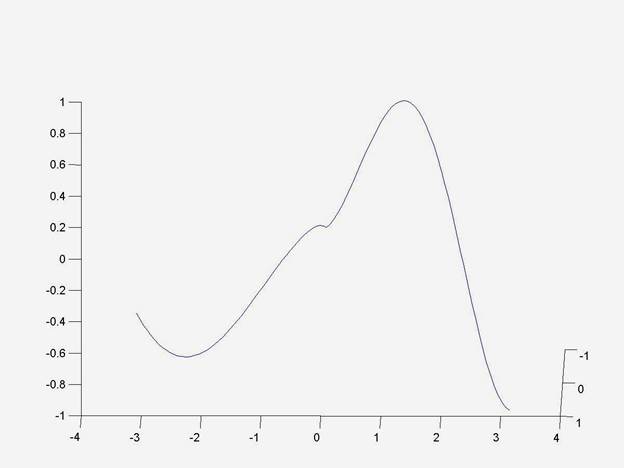
Rotate the camera a bit and you see the kink more clearly:
A second-order discontinuity is very hard to see this way, so first-order continuity is usually sufficient for rendering smooth curves and surfaces.
Further, we can relax the condition a bit by require only that the derivatives have the same direction, but not necessarily the same magnitude. This is called the geometric continuity condition. The condition for zero-order geometric continuity, G0, is the same as that for zero-order parametric continuity: that the curves at the boundary. The G1 condition is that the tangent lines of two successive parametric pieces are parallel. The G2 condition is that the two curves have the same curvature: again, this requirement is usually unnecessary for the purpose of a visually smooth curve or surface. Generally, the a curve meeting the geometric continuity condition, but not the parametric continuity condition will pass through the same control points, but have a somewhat different shape.
For example, if we want to construct a quadratic spline for a curve y = f(x), we can compute coordinates of three points on the curve, say, and then define so that
is a system of equations we can solve for the vector coefficients a0, a1 and a2:
======================================================== For a given set of control points (boundary points) and a degree for the polynomials we want to patch together, there are three main ways to specify a spline:
As an example, a section of cubic spline can be represented as where B is a column vector representing the boundary points and A is the 4x4 transformation to spline form matrix. This is actually what’s termed a change of basis matrix in linear algebra?
We can also think of this as getting a polynomial representation of a particular coordinate (say, y, of (x,y,z)) in terms of the boundary parameters bk by choosing the right blend of polynomials like so: Where Pk(t) are the blending (basis) polynomials.
I’ll admit
that last bit was too slick and quick that correspond to the partition We can reduce the problem to interpolating x(t) using cubic splines with, say, which, conveniently, meets the boundary condition There will be n−1 splices with 3 unknown coefficients per splice, making 2n−1 coefficients to be determined, meeting the other boundary constraints: and, to meet the n−2 first-order continuity constraints, or, in dot-hat notation, For second-order continuity, require that To simplify
notation, let
and first-order conditions are
while the second-order conditions are
Further, the conditions for a “natural spline” require that the curve begins and ends with curvature zero means
Summing up, we have the following system:
For simplicity, here’s the matrix version of this system when n = 3: It turns out the computation can be made more efficient by considering both endpoint of a sub-interval. Consider this form of the cubic spline (note this s is not the s above): The first and second derivatives for k = 1, 2, …, n-1 are Thus
EQ1 contains 3n − 2 unknowns: ai, bi,
and ci for i = 1, 2, … , n − 1 and cn.
We can find bk by applying the zero-order constraint Similarly, we can find the ak by applying the zero-order constraint at the other endpoint: It remains to
get a formula for the ck,
which, as we’ve shown, also represent the values of the second derivatives of
s at the control points. If we apply the first-order continuity
condition whence, for 1 < k < n,
Now, since the formulas for ak and bk both depend in ck, we can substitute to obtain n−2 equations involving only ck-1, ck, and ck+1, for k = 2, 3, … , n − 1
If you then impose the natural spline boundary conditions; that is, that the curvature at the extreme endpoints is zero, then For simplicity, let wk represent the slope so that the equation for ci values can be written as the dot product Together with the natural spline boundary constraints, this can be written in matrix form as Ac = d: Isn’t that impressive?
Tomorrow we’ll maybe look into writing out the pseudocode and some c++ to implement this. |