[page 1, page 2, page 3, page 4, page 5, page 6, page 7, page 8]
More Exercises/problems:We can still perform a phase comparison on a pixel-by-pixel basis between the two succesive SAR images to recover an estimate of average height within each pixel with this repeat-pass approach.
But what if the surface has changed? Can we still recover topography? Can we determine how the surface has changed? The answer to these questions depends on the nature of the change. In the case where the relative positions of the radar scatterers within a pixel changes by amounts greater than the radar wavelength, we are out of luck--phase coherence will not be maintained in the second image relative to the first, and we cannot peform a pixel-by-pixel phase comparison between the first and second image. We cannot recover topography with the single-antenna system, nor can we say anything quantitative about the nature of the change, beyond stating that it has been larger than some minimum value. However, if we had the foresight and resources to acquire our first set of data with a dual-antenna system (thereby obtaining topography on the first pass), we could at least perform a differencing operation on two independent height estimates, obtaining displacement information precise to the several-meter level.
Now consider a second case, where the only surface change is a large-scale coherent change common to several adjacent pixels. By this we mean that, within a given pixel, the position of radar scatterers has not changed to any significant degree, but the ensemble of scatterers (i.e., the entire ground surface within that pixel, as well as some adjacent ones) has moved up, down, or sideways in some correlated fashion. Now we are able to perform a phase comparison of the two images. The differential phase contains information on the range change to the radar antenna, thus providing information on the surface change, precise to a fraction of a radar wavelength, or to a few millimeters to centimeters for typical radars. As discussed in more detail below, to measure surface displacement to this precision requires a relatively accurate a priori estimate of topography in the region and information on the position and orientation of the antennas during each image acquisition.
One measurement of phase change based on two successive images constitutes only one component of the three-dimensional surface displacement vector, specifically the component projected onto the spacecraft-pixel vector. In this respect, it differs from the three-dimensional vector measured by GPS geodesy. The great advantage of SAR is that the observations are acquired with virtually complete spatial coverage, rather than the sparse observations inherent in conventional (including GPS) geodesy. In principle, all three components of surface displacement could be obtained from space; in practice, we are only likely to obtain at most two, if data from both the ascending and descending passes of the satellite are available. Additiona information (e.g., from ground observations) would normally be required to determine the full three-dimensional displacement field. In practice, one or two components will be adequate for most applications.
We have said that measurement of surface displacement with SAR interferometry depends on the nature of the surface change. In fact, the conditions under which SAR interferometry gives useful information on surface change is a major topic of current research. We can restate two important necessary conditions for detecting and measuring surface change with SAR:
The first condition is unlikely to pose significant problems, at least in theory. When it is violated because natural phenomena generate large displacements and displacement gradients (e.g., volcanic eruptions, landslides), simple differencing of before and after topographic data should be adequate to define the changes to the degree of accuracy required for their study. Of course, obtaining such topographic data may be quite challenging in a practical sense.Changes between successive images must not be too large, specifically the displacement gradient across a pixel must fall within some value. The radar-scattering characteristics within each pixel must remain similar in the time between the two image acquisitions, specifically the root-mean-square (rms) position of the surface scatterers within a pixel must remain constant within a fraction,say 10 to 20%, of the radar wavelength. The second condition is more problematic. When this condition is not met, it is termed temporal decorrelation (Zebker and Villasenor, 1992), and it constitutes one of the major problems for SAR interferometry. Temporal decorrelation precludes or makes difficult the phase comparison of the two SAR images. Temporal decorrelation has been observed on time scales as short as a few hours in vegetated areas experiencing windy conditions. On the other hand, the initial result for the Landers earthquake (Massonnet et al., 1993) demonstrated phase correlation over several months in a desert area with no storms. Subsequent studies indicated that phase correlation could be obtained in this arid region over a period of 14 months, from April 1992 to July 1993 (Massonnet et al., 1994). Zebker et al. (1994) and Peltzer and Rosen (1995) describe phase correlation between images taken approximately one year apart in Eureka Valley, California, also an arid region. Qualitatively, we know that desert is better than dense forest, dry conditions are better than wet, and long radar wavelength is better than short, but much work remains to be done in understanding this phenomenon. The Boulder workshop identified temporal decorrelation as a high-priority research topic.
With this as background information, we are now in a position to quantify the concepts and conditions for measuring surface change. Consider again two radar antennas observing the same ground swath as in the figure:
but at different times, as in the repeat-pass mode. The measured phase at each point in each of the two radar images is equal to the sum of a propagation part, proportional to the round-trip distance, and a scattering part due to the interaction of the wave with the ground. If each pixel on the ground behaves the same for each observation, calculating the difference in the phases removes dependence on the scattering mechanism and gives a quantity dependent only on imaging geometry.ISAR#11
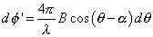
Show how the equation:leads to the approximation
. Justify the validity of the approximation.
ISAR#12
Explain what is meant by callingthe "component of the baseline parallel to the look direction." What is the baseline? What is the look direction? What might another component be?
For the repeat-pass case, we can rearrange
to express the phase observable as
, which is the number of wavelengths in the difference between the distance down and the distance back,
, times
.
If a second (denoted prime) interferogram is acquired over the same area, sharing one orbit with the previous pair so that
and
are unchanged, we can compare the interferogram phases with each other. This second interferogram is acquired with a different baseline length B' and baseline orientation
' thus a different
.
ISAR#13
Show thatand thus that
is just equal to the ratio of the parallel components of the baseline, i.e., independent of topography, since radar wavelength is constant.
Now consider two interferograms acquired over the same region as before but at different times, so that ground deformation (due to an earthquake or volcano swelling) has displaced many of the resolution elements for the primed interferogram in a coherent manner. In addition to the phase dependence on topography, this time there is an additional phase change due to the radar line-of-sight component of displacement .In this interferogram, the phase is
where the surface displacement
adds to the topographic phase term, which could create confusion in the interpretation. However, if the data from the initial unprimed interferogram are properly scaled and subtracted from the primed interferogram, we can obtain a solution dependent only on
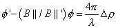
Since the quantity on the left is determined entirely by the phases of the interferograms and the orbit geometries, the line-of-sight component of the displacement is measurable for each point in the scene.Knowledge of antenna baseline length B and orientation
spacecraft and spacecraft orientation during each image acquisition. However, current orbital systems are not designed with interferometry specifically in mind and lack the technology to provide the requisite data. Massonnet et al. (1993) tested a number of satellite passes before finding two with optimum characteristics, then adjusted the orbital parameter estimates to minimize coseismic offset far from the fault. It is also possible to match displacement in the near field with other geodetic data to obtain the necessary constraints. In the future, it is likely that orbital SAR systems will be specifically designed to facilitate acquisition of interferometric data, and thus will include GPS and other tracking techniques to provide accurate information on the position and orientation of the platform.It should be noted that optimum baseline length is a function of radar wavelength and the desired result. For surface change estimates, similar imaging geometry in the before-and-after images is desirable, implying the shortest possible baseline. For topographic estimates, the baseline should be neither too short (reducing sensitivity to surface height) nor too long (causing geometric characteristics of the image to differ by too much and preventing the phases of the two images to be compared interferometrically because they are uncorrelated). Thus, an interferometer designed to recover high-accuracy height estimates represents a compromise between these competing effects. Zebker and Villasenor (1992), Rodriguez and Martin (1992), and Zebker et al. (1994b) discuss this and related design issues. Briefly, for orbital SARs, the correlation between radar echoes varies from unity (perfect correlation) at zero baseline to zero (no correlation) at some critical baseline, Bc
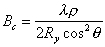
The optimum baseline length is less than Bc and can be determined by minimizing the phase error,
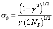
where NL is the number of radar "looks," the parameter
is given by

and signal-to-noise ratio (SNR) is the equivalent thermal SNR--it can contain, for example, quantization noise terms. For
C-band (~6-cm wavelength) ERS-1 SAR data, Bc is 1100 m, the optimum baseline is ~200 m, and antenna separations of 100 to ~400 m can be used to obtain good height estimates.It is important to assess the relative sensitivity of the phase measurement to topography and displacement since the topography itself may be poorly known. The relative sensitivity of the phase may be derived by differentiating
and using
, obtained by differentiating
, we obtain:
and
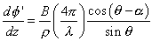
For the displacement case, we have

Since B (a few hundred meters) is much less than
is small. Thus, the measured phase is much less sensitive to topography compared to displacement. Comparing the two results numerically for the case of ERS-1, 1 m of topography gives a phase signature of 4.3deg. (actually less than the real noise limit of ~20deg., implying that ERS-1 is not sensitive to topography at this level). However, for the same pass pair, a 1-m surface displacement yields a phase signature of 12,800deg., or nearly 3000 times greater sensitivity. Since we seek to measure 1-cm surface changes, this implies that we require topographic data accurate to about 3000 x 1 cm, or +/-30 m.
Massonnet et al. (1993) used a preexisting digital elevation model (DEM) in the Mojave Desert that required only two satellite passes (one before, one after) to measure coseismic offset. The DEM for the Mojave region is representative of digital topographic data in existence for most of the Northern Hemisphere (90- by 120-m pixels, nominal vertical accuracy of 30 m); unfortunately, much of it is classified and not available for scientific research. Errors in the DEM contributed about 9 mm of noise to the coseismic offset estimates obtained by Massonet et al. (1993), where rms vertical errors in the topographic data were estimated after the fact to be about +/-24 m. Systematic errors in selected areas can, of course, be much larger than this.
Fig. 2.2. Shows an example of an anomalous feature (rhomboid shape) produced by an error in the digital elevation model (DEM). In this interferogram, constructed from two ERS-1 images acquired in July and December 1992 [Massonnet et al., 1994] , one complete color cycle ("fringe") corresponds to one change in range cycle (28 mm) along the satellite-ground line of site. The four fringes in the rhomboid cannot be attributed to a known earthquake (white dots). Even the largest earthquake during this time period (asterisk) cannot be responsible for the downwelling because of its 7-km-depth thrust mechanism and small 3.9 magnitude. By considering other interferometric pairs, Massonnet and Feigl [1995] attribute the feature to an error of ~250 m in the DEM. One fringe represents 28 mm of range change.
If high-quality DEMs are not available, the topographic data can be derived indepen-dently by the SAR, although three passes are required (the first two generate the height data, the third estimates the change). Zebker et al. (1994a) describe the estimation of the Landers coseismic displacement without reference to a priori elevation data using the three-pass technique. Adequate topographic data can also be obtained from TOPSAR, the NASA aircraft SAR interferometry system (Zebker et al., 1992).
At this time, topographic data of the appropriate quality for change detection are not available for much of the Southern Hemisphere. Thus, it will likely be necessary to use the three-pass approach with ERS-1 and ERS-2 for those observations to generate initial topographic data accurate enough for interferometric change detection. If one considers a space mission optimized to exploit the change-detection capabilities of SAR interferometry, this implies that the first part of the mission (the first 3-4 months) should be devoted to acquisition of high-quality topographic data.
Atmospheric effects are another source of systematic error in surface displacement estimates from SAR interferometry because they change the refraction index, through which the radar signal passes, and thus corrupt the radar phase observable. Tropospheric and ionospheric effects (Figs. 2.3 and 2.4) have both been identified in SAR interferometry images (Massonnet and Feigl, 1995a). Repetitive passes, such as afforded by ERS-1, are probably the best way to separate atmospheric effects from true ground deformation.
Fig. 2.3. An example of a tropospheric effect in two interferograms [Massonnet and Feigl, 1995a] . The image acquired August 27, 1993 at 18:28 UTC is common to both interfero-grams formed with images acquired in December (left) and July (right) of 1992. The irregular circular patterns are 5 to 10 km wide and represent up to 3 fringes of atmospheric perturbation in the August image. One fringe represents 28 mm of range change.
Fig. 2.4. A kidney-shaped feature apparently produced by an ionospheric perturbation in the radar image acquired by ERS-1 on July 3, 1992 near Landers, California. [Massonnet et al., 1994; Massonnet and Feigl, 1995a] . One fringe represents 28 mm of range change.
For another perspective on what is happening to the geology of the area around College of the Desert, visit the Scripps Orbit and Permanent Array Center and read about who they are, what they do, and how they do it. Check out the Permanent GPS Array Sites they have grouped and, in particular, the map associated with Southern California Integrated GPS Network (SCIGN). In the midst of these sites you can easily see "cotd" which is the College of the Desert site. Clicking on the purple diamond for cotd will take you to the cotd information page.
This is the subject of the second part of this unit.