|
Math 2A Vector Calculus
Use
Lagrange multipliers to find the maximum and minimum values of the
function
Let’s
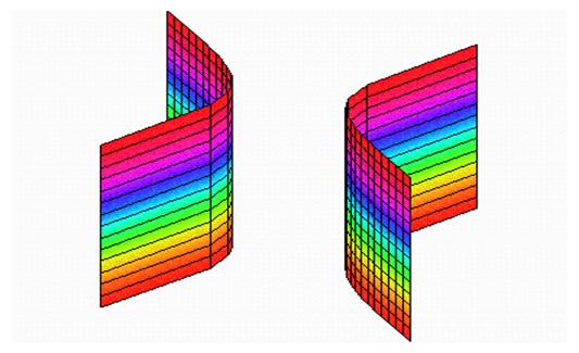
approach the problem through the path of geometric insight. Notice that the first constrain describes
two hyperbolic sheets parallel to the z
In Maple we can plot the two sheets separately using parameterized surfaces as follows:
Then
we can add to this plot the unit cylinder along the x-axis: As seen in the plot3d results shown below we can see the constraint system is visualized as a pair of curvy U-shapes, approaching the lines z = +/-1.
Now
let’s throw in a level surface of our object function. How about w = 2 so that 2 = y(x+z)
means that, after shifting along the z
axis by 3 to avoid discontinuities (one of the niceties of parameterized
surfaces) we have
From this diagram, it does seem like this level surface meets the constraint curve. The trick then, is to pick the value of w where the level surface just barely glances off the constraint curve. To do this, we simply require that the perpendicular vectors (gradients) be coplanar, in the sense that the tangent plane to the level surface is also tangent to each level curve: in other words, the gradient vector for the level surface is a linear combination of the gradients vectors of the two constraint surfaces: So together with the given constraints we have 5 equations in five unknowns:
From
the first equation, λ = 1. Plugging this into the second equation also
eliminates x so that So
evidently, w has a maximum of 1.5
at and a minimum of
0.5 at Let’s try plotting these
to get a feel for what’s going on. In the plot shown you can kind of see the symmetry of plus or minus z values corresponding to the same tangential surfaces.
|