Math 2A Chapter 12 TestProblems
Solutions
1.
Consider the iterated integral
a.
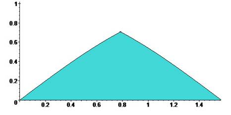
This integral measures the volume under the
surface and over some region R in the tu-plane. The region R is described by the
inequalities
.
Since , The region is sketched below with t as
the horizontal axis and u the vertical axis.
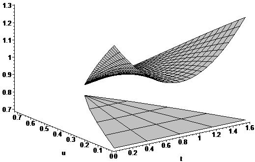
One view of how the surface fits over this region is shown below:
> p1:=plot3d(1+cos(u)-cos(t-Pi/4),t=arcsin(u)..arccos(u),u=0..sqrt(2)/2,color=gray):
> p2:=plot3d([t,u,.7],u=0..sqrt(2)/2,t=arccos(u)..arcsin(u),color=gray,grid=[5,5]):
> display(p1,p2);
b.
Since this last integral doesn’t simplify, we can use numerical methods to
approximate it. In Maple:
> int((arccos(u)-arcsin(u))*cos(u),u=0..sqrt(2)/2);
> evalf(%);
![]()
This
amounts to a volume
c.
Fubini’s theorem applies here because the integrand is
continuous and its first partial derivatives are continuous. Since the surface is symmetrical about the
plane ,
reversing the order of integration leads
to the sum of two identical integrals
,
where the last approximation is from Maple.
This is the same as the result from integrating the other way.
2.
Consider the thin plate bounded by y = x and y = xn
(n > 1) in the first quadrant with density distribution .
a.
The Mass of the laminar plate is The moment about the x-axis is
The moment about the y-axis is
Thus, and
b.
The moment of inertia about the x-axis is=.
The moment of inertia about the y-axis is
c.
Thus and
3.
The transformation , y= v can be used to evaluate
the integral
by first writing it as an integral over a region G in the uv-plane. Clearly, and so
. The Jacobian for this transformation is
. Also,
,
so
.
The transformation , introduces a discontinuity into the domain
and in no way simplifies the integral and so there is no motivation to pursue
it, other than a wild “see what happens” approach.
4.
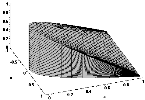
The Maple commands
> p10:=plot3d([x,x^2,z],x=-1..1,z=0..1-x^2,color=gray):
> p11:=plot3d([x,y,0],x=-1..1,y=x^2..1,color=gray):
> p12:=plot3d([x,y,1-y],x=-1..1,y=x^2..1,color=gray):
> display(p10,p11,p12);
can be used to sketch the domain of
integration of the integral ,
as shown below
It can also be expressed as
|
a. |
b. |
c. |
d. |
e. |
Maple can be used to verify that these are, in fact, the
same:
> int(int(int(1,z=0..1-y),y=x^2..1),x=-1..1);
![]()
> int(int(int(1,y=x^2..1-z),z=0..1-x^2),x=-1..1);
![]()
> int(int(int(1,x=-sqrt(y)..sqrt(y)),y=0..1-z),z=0..1);
![]()
> int(int(int(1,y=x^2..1-z),x=-sqrt(1-z)..sqrt(1-z)),z=0..1);
![]()
> int(int(int(1,z=0..1-y),x=-sqrt(y)..sqrt(y)),y=0..1);
![]()
5.
A solid in the first octant is bounded by the planes y
= 0 and z = 0 and by the surfaces and
. It’s density function is
.
a.
The object’s mass is =
b.
.
c.
d.
.
6.
To find the volume of the region bounded above by the
sphere and below by the paraboloid
,
we might start by writing these equations in cylindrical form:
and
. Note that this reduces the number of
variables to 2. Substituting,
so the parabola and the sphere intersect at z
= a and at z = 0. This is
evident in the Maple plot below (where a = 1 is chosen):
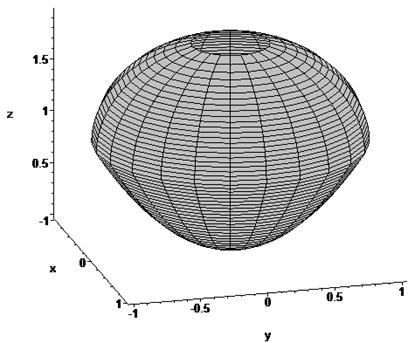
Apparently Maple failed to sample the point at the top, so it looks like it’s
lost its lid!
The volume integral is best set up in either cylindrical or spherical
coordinates. In cylind3rical coordinates
we have
.
In spherical coordinates, observe that the curves intersect z = a
and . Thus
Of course, it might be simpler to compute the volume below the paraboloid and
above the sphere and then subtract that from four thirds pi a cubed.
7.
In cylindrical coordinates, the integral
is
8.
The mass distribution over the region bounded by
,
and
.
a. ..has center of mass .
b.
The moment of intertia about the z axis and the
corresponding radius of gyration.
9.
Find the area of the surface described by