Ex2:
How about taking a string and waving it around on the home screen?
Here's a more complicated program which illustrates a few tricks.
:ClLCD
// Clear the screen
:Degree //
Set degree mode (for sine function below)
:Outpt(4,4,"Enter a string.")
//Prompt for input
:InpSt S //Input
a string into variable S
:ClLCD
// Clear the screen again
:lngth S->N // Measure
the length of S and store in N
:N->dimL L //
L and T will hold coordinates of
:N->dimL T //
characters on the screen.
:For(K,1,N) // Initialize
position arrays
:4->L(K)
// Initial position in middle of screen
:(4,4)->T(K) // T
is the old position - complex format
:End
// is used to keep coordinates as real and imag
:1->A
// Is the degree measure of an angle
:While 1 //
Loop forever - or until [ON] interrupts
:For(K,1,N) // Write
the string
:Outpt(L(K),K+int ((21-N)/2),sub(S,K,1))
// Note horiz. center
:(L(K),K+int ((21-N)/2))->T(K)
// Keep track of old pos.
:A+5->A //Increment
angle to simulate wave motion
:int (5+4*sin (A))->L(K)
// New vertical position
:Outpt(real T(1+mod(K+1,N)),imag
T(1+mod(K+1,N))," ") //erase
:End // End For loop
:End // End While
loop
Try substituting sin
(2*A) for sin (A)
or tweaking other parts of the program. Note that it runs pretty
slowly - can it be sped up?
getKy
and While
The
getKy function checks to see if the user has pushed any
keys. If the user has not, it puts a 0 (zero)
into variable. If a key is pressed, then
getKy puts a value into variable, depending on which key
was pressed. The general form is:
getKy <variable>
Here's a list of keys
and their return values:
[F1]-[F5]:
11-15
[2nd] - [<right arrow>]
21-26
[ALPHA] - [<down arrow>] 31-34
[GRAPH] - [CLEAR]
41-45
[LOG] - [^]
51-55
...and so forth, except that [ON] is not numbered,
so there is no 101.
Using getKy
with the control command, While,
is an effective way to branch a program from user input. Here's a
little program fragment to illustrate this:
:0->M
:While M==0
:getKy->M
:End
:Outpt(4,10,M)
The first command puts
0 in a variable called M.
The While command then executes the
following command(s) (until End) which,
in this case, is the single command to put the value of whatever key is
pressed into M. If no key is
pressed, M is
0 and the while-loop continues. As soon as key is
pressed, M takes the value of that key and the loop is exited. At this
point, the output command will execute. Try it! Use [2nd]
[2] to bring up the test menu where "=="
lives.
Note the relational operator,
"==," should not be confused with
the assignment operator, "=,"
which stores an expression in a variable of type EQU.
The "equals?" operator, ==, checks
to see if two values or strings match, and returns
1 if they match or 0 if
they don't match.
The
If-Then-Else
Controls
The
If function makes decisions in a program based on whether
or not its argument equals zero. If the argument equals anything
but zero, it does whatever is on the next line after If. The general form
is:
:If <argument>
:<stuff done if argument
does not equal zero>
:<stuff done in either
case>
For example,
:If x==3 //x==3 evaluates
to either one or zero
:Outpt(2,1,"Hi Jake")
:DispG
will output "Hi Jake"
only if x holds the value
3. In any case, the graph screen is displayed immediately
afterwards, so you get a chance to see "Hi Jake"!
The word
Then is used after If when
you need more than just one statement evaluated after
If. The word End signals
the end of the list of things to do. This has the form:
:If <argument>
:Then
:<Things to do if argument
does not equal zero>
: . . .
:<Things to do if argument
does not equal zero>
:End
:<Stuff done if If condition
is false>
The word
Else is used to tell the program what to do if argument
does equal zero. It must be used with Then.
It is used after the list of things to do if true (not equal to zero) and
has an End following it. The form
is:
:If <argument>
:Then
:<Commands to do if true (argument
does not equal zero)>
:<Commands to do if true (argument
does not equal zero)>
:Else
:<Commands to do if false (argument
equals zero)>
:<Commands to do if false (argument
equals zero)>
:End
Before we go further, let's take a short course
in how to design code:
The Design
Process
The design process is might be outlined something
like this:
1) Decide what you want your program
to do.
2) Write pseudocode; that is, outline
in broad strokes how the flow will go.
3) Draw graphics, if necessary, on
graph paper - images that the program will use.
4) Work out methods to do difficult
routines, drawing on innovation and experience.
5) Type it in. It's easier to use
a computer keyboard, if you have the Link utility.
6) Test.
7) Debug.
8) Add on new features you think would
enhance the performance.
9) Test
10) Debug
11) Make documentation, bundle, other things
needed for full program.
12) Release beta version.
Ideally, if you can conceive
it (step 1,) you can write it - except that on the TI you are limited by
space, execution speed, and deficiencies in the TI language. Still,
it takes considerably more creativity and imagination to dream up a program
than to write it.
Step 2 refers to writing
on paper, code which uses terms from the language but is just an outline
of what will happen.
Step 3 is necessary
if you want to test parts of the program before it is completed.
If the Pics aren't finished it won't work.
Step 4 is where software
engineers define their skill. You often run into routines you have
no idea how to do. Use pencil and paper so you can see the whole
thing. Make a flow chart, thread through the commands one at a time,
making a list of what variable has what value when. Think of alternatives,
look in the CATALOG for commands that may be useful.
Debugging (aka error
checking or troubleshooting) in step 6 is really an extension of step 4.
This is the "check" part of the "guess and check" method. Sometimes
a bug is so elusive, you cannot find it. This is why professional software
companies release "beta" versions of their software for free. If enough
people try to use the software in crazy ways, its weaknesses usually surface
fairly quickly. Go through the code step-by-step keeping a table
of the values of all the variables involved at those points, and do the
commands just as the TI would. This may help you to see where, when, and
under what circumstances you run into the problem. Try using different
input values: good software is idiot proof and will disallow crazy input.
By the time you've done all that, you may have new ideas, don't be afraid
to start from scratch again.
EX3:
Suppose we dream up an idea to have a character bouncing around the
screen. Recall the program fragment using getKy and
While to get a pressed key's value and output it:
:0->M
:While M==0
:getKy->M
:End
:Outpt(4,10,M)
The program will, as I imagine
it, place an alphabetic character associated with the key in a random position
on the screen and set it in motion down and to the right until it hits
a "wall," at which point it will "bounce" and continue bouncing until another
alphabet key is pressed at which time the new letter will be randomly placed
and start bouncing. To stop the process the [(-)]
key will be used.
So that's step 1 in the
design process. The pseudo code now might look like this:
Initialize screen and variables
Use the While/getKy technique to wait for and
take input
If the key doesn't have an alphabet character,
ignore it.
If the key has an alphabet character, place it
on a random spot on the screen.
While no new key is pressed, and the character
is not at a wall, erase it and
redraw it one spot down and to the right.
Continue this erase/draw procedure until you
get to a wall, then bounce.
Yeah? Now since there
are now graphics to draw, we proceed to step 4. I prefer using the
computer to type in the program pieces as I think of them, but paper is
preferable to trying to type in stuff on the calculator directly.
Rather than start at
the beginning and develop code linearly, it may be better to start in the
middle and work outwards. Can you identify loops that will be employed?
We'll need one loop to accept a character and another to bounce it around
once we have it.
Some languages
have a "case" statement which can be used to branch on a key press, on
the TI, the If-Then-End commands can serve the purpose - but since there
is no methodical way to converting the number value to an alphabetic character
that I can think of, I think I'll need a separate If-Then-End statement
for each key.
Does this mean retyping
the code for moving the character inside each Then-End block? Fortunately,
no. We can write what's called a "subroutine" as a separate program
which can be called by the main program. Let's see how this might
work.
Given the alphabetic
character, the subroutine will need to to choose its initial position and
send it moving with erase/redraw. It will also have to know when
a new key is pressed. Finally, it will need a way of moving the figure.
Assuming the alphabetic character has already been stored in the variable,
S, after some fumbling, I come up with:
:1+int (20*rand)->H
// Choose a random integer between 1 and 21
:1+int (7*rand)->V
// Choose another between 1 and 8 (inclusive)
:1->I //
These are the increment variables, initially set to
:1->J // move
the character down and to the right.
:0->M // M will hold
the value of any key that is pressed.
:While M==0
// If a key is pressed, we'll exit the subroutine
:if H==21
// If at the right wall,
:-1->I
// then reverse the horizontal increment (bounce)
:if H==1
// If at the left wall,
:1->I
// bounce right.
:if V==8
// If at the bottom,
:-1->J
// bounce up.
:if V==1 //
If at the top,
:1->J
// bounce down.
:Outpt(V,H," ")
// Before incrementing the indices, erase.
:H+I->H
// Increment horizontal position.
:V+J->V
// Increment vertical position.
:Outpt(V,H,S) //
Redraw the character at the new position
:For (K,1,30) //
Kill some time (if it moves too fast, you can't see it.)
:1->N
// Whatever...
:End
// End For loop
:getKy->M
// Check to see if a key has been pressed
:End
// End while loop
:Return //
Go back to the main routine.
Enter this code under
the name POSSUB.
Now all we need is a
routine which will see which key has been pressed and convert its value
to an alphabetic character. The following gets the job done, even
if it looks a bit clunky:
:ClLCD
:1+int (20*rand)->H //
Initialize the horizontal position.
:1+int (7*rand)->V //
Initialize the vertical position.
:0->next //
When next is 1, we exit.
:ClLCD //
Clear the deck.
:0->M
:While (M==0) //
Wait for the first key press to get going.
:getKy->M
:End
:Repeat next
// This is the outer loop of the main routine.
:Outpt(1,1,"HEY")
// This was originally for error checking - I left it in.
:Outpt(3,1,M)
:If M==51
// If the value of the key pressed is 51
:Then
:"A"->S
// The "A" key was pressed so load S with "A".
:POSSUB
// Do subroutine stuff with "A" in S.
:End
:If M==52 //
Same as above, only the "B" key was pressed.
:Then
:"B"->S
:POSSUB
:End
....
// Repeat If-Then-End for each character of the alphabet.
:If M==103
:Then
:"Z"üS
:POSZ
:End
:If M==105 //
If the [ENTER] key is pressed
:Then
:1->next //
Load next with 1 so as to exit the Repeat loop.
:End
:End //
End Repeat loop.
The Repeat function does
a series of commands, then checks if a condition is true (does not equal
zero). It differs from While in that the <Things to do again if condition
is true> get done at least one time, regardless of whether or not the condition
is true. Repeat will also create an infinite loop without help if condition
is true initially. The While and Repeat functions are just For() loops
that don't increment (increase by a value every time around) conditions
themselves.
The
IS>() and DS<()
Commands
The
IS<() (increment and skip) command increments the variable
by one and skips the next command if variable is greater than <value>
. This function has the form:
:IS>(<variable>, <value>)
:<Command to skip if
variable exceeds value>
The
DS>() (decrement and skip) command decreases the variable
by one and skips the next command if the variable is less than <value>
. This function has the form:
:DS<(<variable>, <value>)
:<Command to skip if
variable is less than value>
The
Lbl and Goto
Commands
The
Lbl and Goto functions
allow the program to go to a certain part of the program that has been
Lbled. For example,
:<commands>
:Lbl <labelname> ...to
here.
:<commands>
:Goto <labelname> Control
goes from here...
:<commands>
The
Menu() Command
Getting
Maximum Graphics on the '85.
Say you're writing a
game which involves a bouncing ball. You could use Outpt(x,y,"o ")
to make the ball and form a paddle with \. This is easy, but
higher quality images require using the graph screen. Using the PtOn (X,
Y) command, a program can draw an image point by point. To create
graphics point by point is extremely time consuming at the production stage,
but it is the secret to the beautiful graphics.
Using
the Graph Screen for Animation from a Program
We've already seen animation
on the home screen. Animation on the graphics screen is just as easy,
but much more powerful. Instead of drawing a character at a time,
we achieve much higher resolution by drawing a pixel at a time, and much
more flexibility by drawing from a library of pre-drawn pictures.
Image drawing algorithms can be relative to a variable point, so the same
subroutine can be used to draw a "pic" anywhere on the screen. Each
PtOn command takes some time to execute (though, if the PtOn's are chained
together, the total time is not a simple multiple of the the time to perform
a single PtOn) so the game is to get the job done with a minimum of commands
- this allows you more control over the speed the program runs. That
is, you can always slow it down by inserting dummy commands, but speeding
up is _not_ always possible.
Using
Line() and PtOn() in
cases where the pic will only require less than, say,
50 pixels is preferable to using ClDrw
or RcPic which effect
all 127*63 = 8001 pixels. In
cases where more pixels are present, StPic does
a better job at keeping things small. And, don't ever forget to set xMax
at 127, yMax at 63, and xMin,yMin at 0.
The
Graph Tools
The
Line() function draws a line between
(x1,y1) and
(x2,y2). Line()
requires less time than PtOn() if
more than one point needs to be turned on - and Line()
takes up less memory than several
PtOn()s. The syntax for
Line() is:
The
PtOn(x,y) function "turns on" (darkens) the pixel at
(x,y). Avoid PtOn() in
cases where Line() will do. The
PtOff(x,y) function is like PtOn, but it makes pixels light
(off).
Since the Outpt() command
doesn't write to the graph screen, to print text on the graph screen requires
drawing the character using the Line() and
PtOn() commands.
Make a grid (or use graph
paper) the size of your desired letter or number. Write y,y+1,y+2,...
in a column on the left side of the grid, and
x,x+1,x+2,... along the bottom. Then, fill in the boxes
(corresponding to pixels) to draw the letter. For example:
y+5 ž
y+4 ž ž
y+3 ž ž
y+2 žžžžž
y+1 ž ž
y ž ž
xxxxx
++++
1234
A short program (say, DrA)
to draw this letter could be:
:1->xMin
// Set the graph window so that
:1->yMin
// each integral value of x and y
:63->yMax
// corresponds to a unique
:127->xMax //
pixel.
:FnOff
// Unselect all functions.
:Prompt x,y //
Quick easy way to get input for position
:Line(x,y,x,y+3)
:PtOn(x+1,y+4)
:Line(x+2,y+5,x+4,y+3)
// Draw "A" on the graph
:Line(x+4,y+2,x+4,y)
// screen.
:Line(x+1,y+2,x+3,y+2)
Note that it's dangerous to use "x"
here since this is a variable the '85 writes to often. Hey, we're learning
- live dangerously! Just watch out later on!
 When designing a full-screen graphic to be saved as a
Pic, make a 127 x 63 grid.
If you have access to a computer graphics software like Photo Shop Pro
or Paint for Windows, make a 127 x 63 rectangle
and use the software tools available to draw the picture, then transfer
to graph paper with a pencil. Then on the TI use the [PEN]
tool under the [GRAPH] [MORE] [DRAW] [MORE] menu.
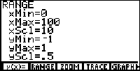
If your range is set as in the DrA program
above, you will see the exact coordinates of the pixel the cross hair is
on at the bottom of the screen. Maybe this is how the Dilbert graphic shown
here was made? I don't who did it, or where I got it. Below is the Photo
Shop prototype of Cyclops with Birds I created, together with the TI Pic
I made from it:


Note that I got confused by the coordinate system
of Photo Shop (which has y increasing as you go down) so the first bird
is too low. Also, I ad-libbed a bit in the translation. Just
impatient, I guess.
Better yet, in many ways,
is the 86iview program available for free at the TI calculator archives:
http://www.ti.com/calc/docs/arch.htm. Using 86iview I drew the following
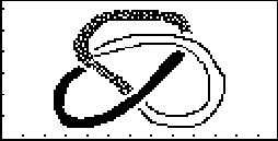
picture demonstrating the 3-colorability of the trefoil knot, in 2 minutes:

Execution
Times (times are in thousandths of a second.)
For Loop_______________________________5.50
PtOn__________________________________18.89
PtOff_________________________________16.55
10 PtOns______________________________25.63
10 PtOffs_____________________________25.62
Line (1,1 to 1,1)_____________________28.89
Line (1,1 to 127,63)__________________52.67
Chain of PtOns from 1,1
to 127,63___3255.01
Circl radius 1______________________4137.16
radius 30___________________________4504.17
If____________________________________12.68
If-Then-End___________________________13.42
ClDrw__________________________________0.73


 COMPLEX:
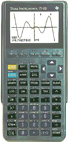
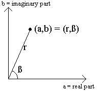
The '85 has a built in complex number type. In the rectangular form
(a,b) that represents the complex
number a+bi where a
and b are real numbers and i
is the imaginary unit whose square is -1.
Complex numbers can also be represented in polar form as
(r,ß) where r is
the modulus and ß is the angle.
Complex numbers can be added, multiplied, etc. like real numbers and there
are some additional operations: conj gives
the conjugate; real gives the real
part; imag gives the imaginary part;
abs gives the modulus; angle
gives the angle.

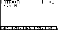
 Type rSwap(A,1,4)->A to swap the rows
1 and 4.
This is an easy way to get a "1" in
the 1st row/1st column position.
 Now do mRAdd(-4,A,1,2)->A to add
-4 times the first row to the second row.
 To finish off the first column add -5 times
the first row to the fourth row with mRAdd(-5,A,1,4)->A.
Ok? First column complete!
 Now multiply the second row by -1 to
get a 1 in the 2nd row/2nd column
position: multR(-1,A,2)->A.
Subtract the second row from the third.
 Subtract twice the second row from the fourth row. So far we've been
able to avoid fractions, but now we have a bit of a problem. This could
be handled in a number of different ways.
 Dividing the last row by 4.2 shows
that z=10. Back-substituting
yields the other solutions: y=4, x=-3 and
w=2.
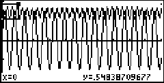 Note that we have too many oscillations and there are no points of intersection
below the axis, so I've created a zoom box on a portion around the upper
left where there may be some intersection. The coordinates of the lower
left corner of the zoom box are shown at the bottom of the screen.
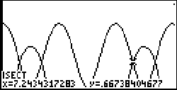 After zooming in, you could simply trace and zoom again for accuracy -
I pressed [MORE] [F1] [MORE] [F5] to
initiate the ISECT function moved
the cursor some and pressed [ENTER] twice
and '85 came up with the point of intersection shown at left. Notice that
the third of four points of intersection in this window is highlighted.
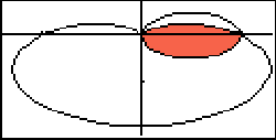 What if we want to find the area common to the interiors of these closed
curves? To see this area on you '85, hit the r(θ)=
key and set r1=cosθ
and r2=1-sinθ
and then [GRAPH]. With
the ranges set for θMin=0 θMax=6.2832,
xMin=-1.4, xMax=1.4 we get the graph shown here (color is added
to the overlapping region by Photo Shop - the Shade
feature only works on the rectangular page.) Another
awkward gap is that you can't measure areas with the integrating function
as you can on the rectangular page.
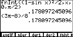 Adding in the area of the half circle we have a total area of
pi/2 - 1. Here's a screenshot of my check on the '85 at
left - just checking that the portion of the area enclosed by the cardioid
is right. fnInt is the numerical integrator which is accessible by pressing
[2nd] [<division>] to bring up the calculus menu, and
then [F5].
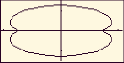 and
then [2nd] [F5] to see the graph use
zoom box or set the range to tMin=0, tMax=6.28, xMin=-1.1,
xMax=1.1, yMin=-1.5, yMax=1.5 and you'll see a peanut-shaped
graph. This is the shape employed by the rotary engine. To compute various
pressures inside the engine, you need to compute the area enclosed by the
epitrochoid. It is extremely difficult (if not impossible) to express this
shape in rectangular or polar form - fortunately, we don't need to. To
compute the area in the first quadrant, simply integrate
Sxdy = Sx(t)(dy/dt)dt =
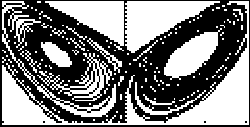 From the [GRAPH] menu push
[F3] to set the initial conditions as say, QI1=-10;
QI2=-10; QI3=30 and from [F2] set
the range as tMin=0; tMax=50; tStep=.01; tPlot=0;
xMin=-15; xMax=15; yMin=10; yMax=40. Also with
[F4] choose axes: x=Q1; y=Q3.
Finally, hit [F5] to graph and kick
back for about 30 minutes.
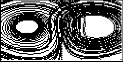 Here's a picture of the same system with the same initial conditions, only
viewing the plot of x=Q2; y=Q3. From
these two projections you can imagine what the 3-dimensional graph might
look like. To see a picture of it and read some more about how Lorenz used
this system to model air flow inside a heated box, check out this site:
http://www.students.uiuc.edu./~ag-ho/chaos/lorenz.html
 EX1:
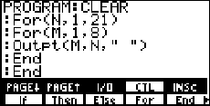
You can erase a value off the screen without clearing other values by using
Outpt to put blank space(s) at that location. See how this
technique can be combined with nested "for" loops to clear the screen.
Press [PRGM] [F2] to bring up program
edit and then type CLEAR (using the
blue keys) then use the [I/O] and
[CTL] menus to type in the code shown on the screen shot
at right. [EXIT] twice to save the
program. Load up the home screen with some flotsam and jetsam, press
[PRGM] [F1] to bring up the program names menu and hunt
for "CLEAR" (using
[MORE] if necessary) and peck it. It's a nice illustration
of how nested "for" loops work.
 When designing a full-screen graphic to be saved as a
Pic, make a 127 x 63 grid.
If you have access to a computer graphics software like Photo Shop Pro
or Paint for Windows, make a 127 x 63 rectangle
and use the software tools available to draw the picture, then transfer
to graph paper with a pencil. Then on the TI use the [PEN]
tool under the [GRAPH] [MORE] [DRAW] [MORE] menu.
If your range is set as in the DrA program
above, you will see the exact coordinates of the pixel the cross hair is
on at the bottom of the screen. Maybe this is how the Dilbert graphic shown
here was made? I don't who did it, or where I got it. Below is the Photo
Shop prototype of Cyclops with Birds I created, together with the TI Pic
I made from it:


