Math 1A – Chapter 2 Test Solutions – Fall ’04 – Pr. Hagopian

1.      Consider

a.       Approximate the value of  at x = 64.001 and 63.999 – what do your results suggest about ?   SOLN: 
, in significant digits:  3.0000
, in significant digits:  3.0000
Which strongly suggests that .

b.      How close does x have to be to 64 to ensure that the function is within 0.1 of it’s limit?

SOLN:  We want to choose a distance δ small enough to be sure that if  then .  It turns out this gives great latitude for δ.  It is appropriate to use the SOLVER on the TI85 (see screen shots below), by which we find that f(x) = 2.9 near x = 42.0929 = 64 – 21.9071 and f(x) = 3.1 near x = 93.8937 = 64 + 29.8937, so that, if x is not much farther than 21.9 units from 64, then f(x) will be within 0.1 units of 3.    Note also that

2.      Is there a number a such that   exists?  If not, why not?  If so, find the value of a and the value of the limit.
SOLN: Since the denominator of  has a zero at x = 1, we need to require that the numerator also has a zero at x = 1; that is, 2+a+a = 0 or a = –1.   To be sure,

3.      Consider .

a.       What theorem is essential to evaluating this limit.  Why are the conditions of the theorem met?
The relevant theorem says that if   (i.e. the limit exists) and if f is continuous at b (i.e.  ) then .  Since  is a composition of continuous functions, it is also continuous, thus the conditions of theorem are met.

b.      Use the theorem to evaluate the limit.   SOLN:
 

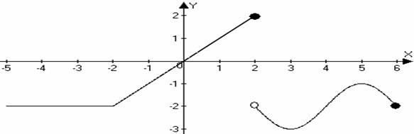
4.      For the function g whose graph is shown, approximate the following, writing “DNE” if the limit doesn’t exist and  or , as appropriate. 

a.    horizontal asymptote	b.	c.
d.    , DNE	e.	f.

5.      Suppose the height H of an object (in meters) at time t (in seconds) is given by

a.       What is the average velocity over the interval
SOLN:  m/s.

b.      Find an interval over which the average velocity of the object is a 1000 m/s.
SOLN:  Since the jump discontinuity has an instantaneous change which is infinite, it shouldn’t be to hard to find a relatively puny rate of change like 1000 m/s.  Fix one point at (0,1) and a variable point (t,0) preceding that point.  Then the average rate of change is .

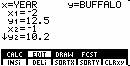
6.      Let B(t) be the number of Elbonian buffalo per capita at time t.  The table below gives values of B(t) as of June 30 of the specified year.  What is your best approximation to the value of ? 

SOLN:  Averaging the immediate before and after rates of change leads to  buffalo per capita per year, but this doesn’t take into account the data from 1998 and 2002.
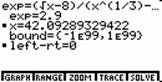
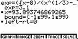
Let’s see if we can include these data.  One way is to fit a quartic function to the data, which can be done by substituting the t, B pairs into the general form .

You could go ahead and solve the 4x4 system this leads to, or you could get the same result by using the TI85, say, to do “regression analysis” on the data.  Start by entering the data using the STAT interface. See the first screen shot.  Note that the t values are taken as years since 2000, ranging from -2 to 2.  This is done to make the computations more stable.   Then choose the P4REG calculation which shows that

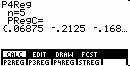
   and thus in year 2000 we estimate  buffalo per capita per year, which is about half the rate of change computed with the previous method…but a whole lot more trouble!  It can be argued that the extra trouble does produce a more accurate measure, but is there an easier method of computing it?  You bet—and it’s a subject of intense interest.  See, for instance, the paper at http://webpages.dcu.ie/~carrollj/202-ln-b.pdf .  As a typical starting point, one would form a forward difference table:            
                      

 

7.      Consider the function .

a.       Use the definition of the derivative to show that .   SOLN: 

b.      Find an equation for the line tangent to x(t) where t = 1.
SOLN:  We plug into point-slope form:

c.       Use a linear approximation to approximate x(1.05)
SOLN: 

8.      For the function  whose derivative function  is graphed below, find where:

a.        is increasing if , which is true for

b.       is concave up where  is increasing, that is,

c.        has a local maximum(?)   SOLN:  This question turns out to be more interesting than intended.  In fact, the graph given contains contradictory information about the derivative function where x = 2: it can’t be true that the derivative function is defined there and yet has a jump discontinuity.  That would mean that f has a tangent line at a point where the slope changes abruptly—can’t be!  Disregarding the nonsense definition of , f  may or may not have a maximum where x = 2, depending on whether or not f(2) is defined and whether that definition leads to a maximum or not.

d.       is positive. . SOLN: This is equivalent to part (b).  is concave up if  is increasing, which is true true for

e.       .  SOLN:   changes from decreasing to increasing where x = 3, and from increasing to decreasing at x = 5.  at both of these points,  is smooth/differentiable so .  While  changes from increasing to decreasing at x = 2, it does so abruptly so that  is undefined.